Why genome completeness and contamination estimates are more complicated than you think

Genome-resolved metagenomics is the process of recovering de novo genomes belonging to individual organisms present in a community using DNA extracted from the whole community. These genomes are sometimes referred to as MAGs (metagenome-assembled genomes), and are recovered by associating assembled contigs together in “bins” in a process known as genome binning. As opposed to traditional genome sequencing, where DNA from an isolate culture is sequenced and used to assemble a genome, when recovering MAGs there is the potential of introducing DNA into a genome bin that shouldn’t be there. Therefore, with MAGs especially, it is important to determine how complete and contaminated recovered genome bins are.

The most common way of assessing the quality of genome bins is to identify and count universal single copy genes (SCGs). Universal SCGs are those which are found in all known life, and in only one copy. Several lists of single copy genes exist (Creevey et al., 2011; Parks et al., 2015), and they mainly consist of genes encoding for ribosomal proteins and other housekeeping genes. Using these lists, you can get an idea of the completeness and contamination of a de novo bacterial bin. Roughly, completeness is the number of unique SCGs present within the bin / the number of unique SCGs in the list. Contamination is estimated by looking at how many SCGs are present in multiple copies, as only one copy should be present of each SCG per genome. Currently, CheckM is the program most often used to assess completeness and contamination (Parks et al., 2015).

While the calculation of completeness and contamination based on SCGs is pretty intuitive, a non-intuitive but important aspect of the calculation is the fact that this method only works well when genomes are relatively complete. This is due to a bias resulting in completeness being overestimated and contamination being underestimated in incomplete bins. To quote Parks et al.:

 

The bias is the result of marker genes residing on foreign DNA that are otherwise absent in a genome being mistakenly interpreted as an indication of increased completeness as opposed to contamination.

 

To illustrate this point with an example, imagine Genome_A that contains 10 unique SCGs out of a list of 50 SCGs. That means Genome_A is 20% complete and 0% contaminated. Now imagine a second genome, Genome_B, with 5 SCGs. If we were to combine the contigs of Genome_A and Genome_B what should ideally happen is we should find that the combined bin, Genome_AB has a contamination increase of 10% with completeness that remains unchanged. However, because Genome_A is only 20% complete, it is very likely that at least some of the 5 SGCs in Genome_B would be different from the 10/50 that were already in Genome_A. This means that in reality the completeness could go up to 30% and the contamination could stay at 0%. This is bad, and illustrates the danger of assessing the completeness and contamination of incomplete genomes.

Now imagine Genome_A with 40 unique SCGs out of a list of 50. That means this genome is 80% complete and 0% contaminated. If 5 more SCGs were selected at random and added to Genome_A, it is probabilistically very likely that at least some (or all) would overlap with the 40/50 already present in Genome_A. This will result in a bin with 40 SCGs, 5 of which are now in duplicate copy. That means the completeness will still be 80%, but the contamination will now be 10%. This is good, and illustrates the utility of SCG analysis.

If you’re thinking that you could fit a binomial distribution to this in order to calculate the extent of this bias, you are right. Below is supplemental figure S8 from Parks et al.

 

 

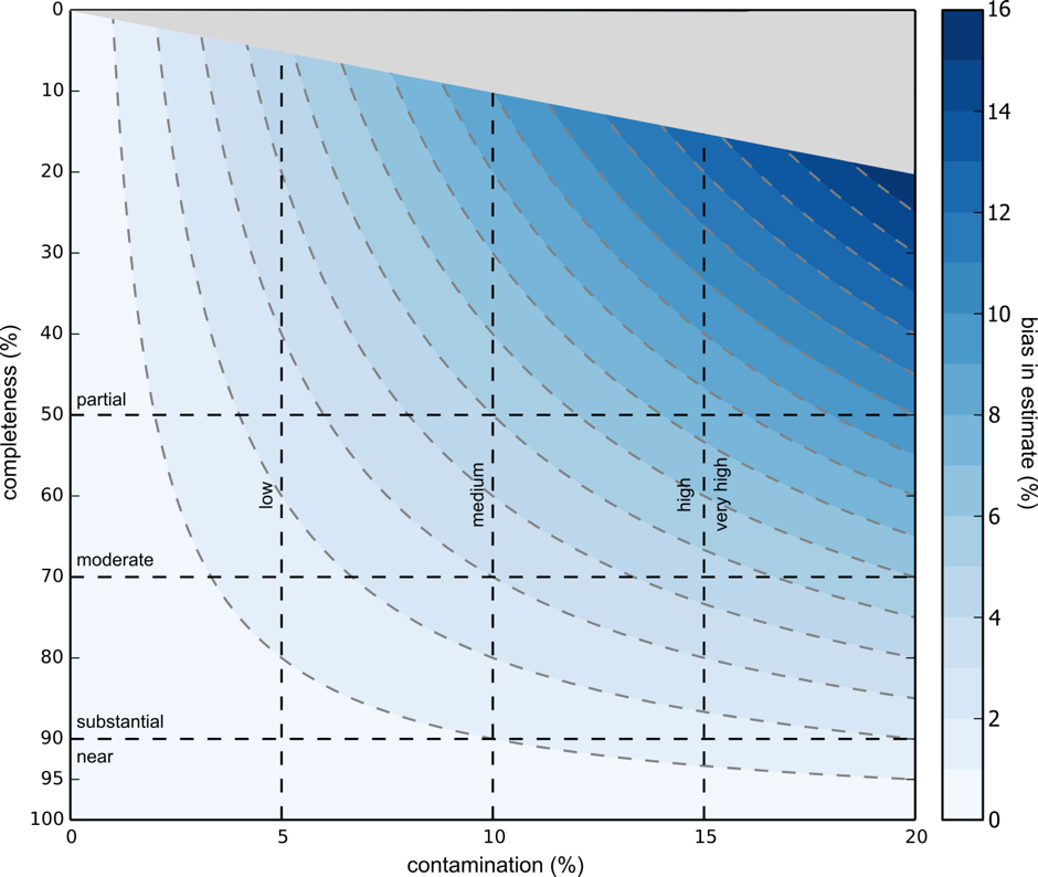
As shown above, higher completeness results in lower systemic bias in completeness and contamination estimates. This bias is very small (<2%) in cases where genomes are over 70% complete and less than 5% contaminated, and OK (<5%) in cases where genomes are over 50% complete and less than 10% contaminated.

As a final example of what happens when you do use genomes with low completeness, below is a figure from a recent paper published in Frontiers in Microbiology (Becraft et al., 2017).

 

 

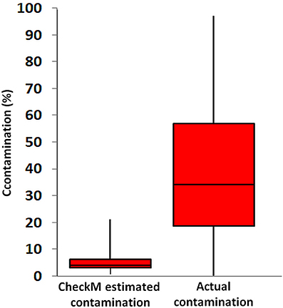
To generate this figure, the authors randomly combined genomes generated using single-cell genomics (SAGs), to test how well single copy genes could estimate artificially introduced contamination. SAGs ideally address the issue of contamination by being assembled from a single microbial cell, but resulting genomes are often very incomplete (~ 1 – 40% complete) due to the limited amount of DNA that can be extracted and amplified from a single cell, leading to incomplete yet potentially pure genomes. After randomly combining these incomplete SAG genomes, the authors then calculated the true contamination of each combined genome by considering the fraction of DNA in a combined genome they knew to come from an artificially introduced set of contigs. They then compared the output of checkM (SCG analysis) on the SAGs individually vs the known contamination created through random merging of bins.

The above figure suggests that checkM is not able to accurately estimate genome contamination in these combined SAG genomes. This is entirely dependent on the fact that these single-cell genomes are very incomplete (they range from 1-40%). While CheckM is able to accurately identify true levels of contamination in highly complete genomes, in genomes that are both fragmented and contaminated the probability of obtaining a contaminating marker gene as a duplicate quickly decreases.

There are also some more subtle things going on in the figure. CheckM presents contamination as the percentage of the expected number of single copy markers that were duplicates, not as a percentage of the obtained genome. A genome bin with just two copies of one SCG out of a list of 50 expected SCGs is 100% contaminated based on the percentage of the obtained genome, but only 2% contaminated based on the percentage of the expected genome. In the above figure, “CheckM estimated contamination” is based on a percentage of the expected genome, and “Actual contamination” is based on percentage of the obtained genome. This accounts for about half of the difference between checkM and the true contamination by itself.

A final note: there are cases where it is perfectly valid to use genomes with low completeness estimates. For example, when it is certain that all DNA originates from the same known organism and introduction of foreign DNA is not a concern (isolate sequencing and single-cell genomics in the absence of contamination). Additionally, there are other ways besides SCG analysis to evaluate the quality a MAG. For example, one could look at time series data and use different clustering methods, e.g. ESOM, to determine the likeness of scaffolds belonging to a bin. SCG analysis is just one way to analyze the quality of a genome bin, and it should always be viewed in the greater context of how the bin was made.

 

-Matt Olm and Spencer Diamond

Banfield Lab

 

References

Becraft, E.D., Woyke, T., Jarett, J., Ivanova, N., Godoy-Vitorino, F., Poulton, N., Brown, J.M., Brown, J., Lau, M.C.Y., Onstott, T., et al. (2017). Rokubacteria: Genomic Giants among the Uncultured Bacterial Phyla. Front. Microbiol. 8, 2264.

Creevey, C.J., Doerks, T., Fitzpatrick, D.A., Raes, J., and Bork, P. (2011). Universally Distributed Single-Copy Genes Indicate a Constant Rate of Horizontal Transfer. PLOS ONE 6, e22099.

Parks, D.H., Imelfort, M., Skennerton, C.T., Hugenholtz, P., and Tyson, G.W. (2015). CheckM: assessing the quality of microbial genomes recovered from isolates, single cells, and metagenomes. Genome Res. 25, 1043–1055.